Since trigonometric functions are also subject to being evaluated for their limit and derivative (you’ll learn more about this in your Calculus classes), we must understand their limits.
This means that we can observe the behavior of different trigonometric functions as they approach different values through the formulas and properties used in evaluating the limits of trigonometric functions.
Limits of trigonometric functions, like any functions’ limits, will return the value of the function as it approaches a certain value of $\boldsymbol$.
In this article, we’ll focus on the trigonometric functions’ limits, and in particular, we’ll learn the following:
We’ll also be applying what we’ve learned in our Trigonometry lessons and also our previous lessons on limits, so make sure to have your notes handy while going through this article.
We can evaluate trigonometric functions’ limits by using their different properties we can observe from their graphs and algebraic expressions. In this section, we’ll establish the following:
Let’s take a look at the graphs of $y = \sin x$ and $y = \cos x$ as shown below.
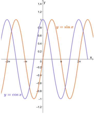
We can see that as long as $a$ is within each function’s domain, the limit of $y = \sin x$ and $y = \cos x$ as $x$ approaches $a$ can be evaluated using the substitution method.
This also applies to the four remaining trigonometric functions – keep in mind that $a$ must belong to the given function domain. This means that when $x = a$ is a vertical asymptote of $ y = \tan x$, for example, the method is not applicable.
Limits of Trigonometric Functions as $\boldsymbol$
Let’s summarize these limits in a table:
| $\boldsymbol <\lim_f(x)>$ | |
| $\lim_ \sin x = \sin a$ | $\lim_ \csc x = \csc a$ |
| $\lim_ \cos x = \cos a$ | $\lim_ \sec x = \sec a$ |
| $\lim_ \tan x = \tan a$ | $\lim_ \cot x = \cot a$ |
As can be seen from the graphs of $y = \sin x$ and $y = \cos x$, the functions approach different values between $-1$ and $1$. In other words, the function is oscillating between the values, so it will be impossible for us to find the limit of $y = \sin x$ and $y = \cos x$ as $x \pm \infty$.
This argument will also apply to the rest of the trigonometric functions.
Limits of Trigonometric Functions as $\boldsymbol$
| $\boldsymbol <\lim_f(x)>$ | |
| \begin\lim_ \sin x\\ \lim_ \csc x \end | Limits do not exist for all six trigonometric functions. |
| \begin\lim_ \cos x\\ \lim_ \sec x \end | |
| \begin\lim_ \tan x\\ \lim_ \cot x \end | |
These are the most fundamental limit properties of trigonometric functions. Let’s go ahead and dive into more complex expressions and see how their behaviors look like as $x$ approaches different values.
The Squeeze Theorem plays an important role in deriving trigonometric functions’ limits, so make sure to review your notes or the linked article for a quick refresher.
We’ll also utilize the limit laws and algebraic techniques to evaluate limits in this section, so make sure to review these topics as well.
Through higher math topics and the Squeeze theorem, we can prove that $\lim_ \dfrac = 1$. This is one of the most used properties when finding the limits of complex trigonometric expressions, so make sure to write this property down.
We can see that it will be impossible for us to evaluate $\lim_ \dfrac = 0$ using the substitution method.
Let’s instead manipulate $\dfrac$ by multiplying its numerator and denominator by $ 1 + \cos x$.
Simplify the numerator by using the difference of two squares property, $(a – b )(a + b) = a^2 -b^2$, and the Pythagorean identity, $\sin^2 \theta = 1 – \cos^2 \theta$.
Since we only have $\lim_ \dfrac$ to work with, let’s separate the expression with $\dfrac$ as the first factor.
We can apply the product law, $\lim_ [f(x) \cdot g(x)] = \lim_ f(x) \cdot \lim_ g(x)$. Use $\lim_ \dfrac = 1> and substitution method to evaluate the limit.
Hence, we’ve just derived the important limit property of trigonometric functions: $\lim_ \dfrac = 0$.
We have two more important properties that we’ve just learned from this section:
With the use of the limits of our six trigonometric functions, the two special limits that we just learned, and our knowledge of algebraic and trigonometric manipulation, we’ll be able to find the limits of complex trigonometric expressions.
Why don’t we test this and apply what we’ve just learned by evaluating more trigonometric functions shown in the next examples?
Example 1
Evaluate the value of the following if the limits exist.
From the form the three trigonometric expressions, it would be a good guess that we might be using $\lim_ \dfrac = 1$. The challenge lies in rewriting the three expressions in the form of $\dfrac$.
Starting with $\lim_ \dfrac$, we can let $u$ be $6x$.
When $x \rightarrow 0$, $6x$ also approaches $0$. This also means that $u \rightarrow 0$.
Rewriting the expression in terms of $u$ and using the property, $\lim_ \dfrac = 1$, we have the following:
Why don’t we apply a similar process for the second function?
If $u = 2x$ and $x \rightarrow 0$, we have the following:
By rewriting the expression of our given, we can now evaluate its limit as $x$ approaches $0$ as shown below.
The third one is a bit trickier since we’ll need to manipulate the expression algebraically, so we can apply the limit formula that what we already know: $\lim_ \dfrac = 1$.
Let’s begin by rewriting $\dfrac$ as a product of $\dfrac$ and $\dfrac$.
We can rewrite the expression by applying the following limit laws:
The table below summarizes how $\lim_\dfrac$ and $\lim_\dfrac$ can be evaluated by rewriting $m$ as $7x$ and $n$ as $9x$.
| $\boldsymbol<\lim_\dfrac>$ | $\boldsymbol<\lim_\dfrac>$ |
| $\begin m &= 7x\\ \dfrac&= x \end$ | $\begin n &= 9x\\ \dfrac&= x \end$ |
| As $x \rightarrow 0$, $7x \rightarrow 0$, and consequently $m \rightarrow 0$. | As $x \rightarrow 0$, $9x \rightarrow 0$, and consequently $n \rightarrow 0$. |
| $ \begin \lim_ \dfrac&=\lim_ \dfrac<\dfrac>\\&= 7 \cdot \lim_ \dfrac \\&= 7 \cdot 1\\&= 7\end$ | $\begin \lim_ \dfrac&=\lim_ \dfrac<\dfrac>\\&= 9 \cdot \lim_ \dfrac \\&= 9 \cdot 1\\&= 9\end$ |
We used a similar approach from the previous item to evaluate the two limits. Since we now have $\boldsymbol<\lim_\dfrac = 7>$ and $\boldsymbol<\lim_\dfrac = 9>$, we can substitute these expressions into our main problem, $\lim_ \dfrac\cdot \left(\lim_\dfrac\right)^$.
Recall that $a^$ is equal to $\dfrac$.
Example 2
Evaluate the limit of $\dfrac$ as $x$ approaches $0$.
The substitution won’t apply to this problem, so we should use a property we already know. The closest that we might have is $\lim_ \dfrac = 0$ since $\sec x$ and $\cos x$ are each other’s negative reciprocal.
Let’s rewrite $\sec x$ as $\dfrac$. Multiply the new expression’s numerator and denominator by $\cos x$, and let’s see what happens.
We can rewrite $\dfrac$ as a product of two factors: $\dfrac$ and $\dfrac$.
Hence, we have $\dfrac = 0$.
Example 3
Evaluate the limit of $\dfrac$ as $x$ approaches $\dfrac<\pi>$.
Let’s first see if we immediately substitute $x = \dfrac<\pi>$ to find the limit of the expression.
This confirms that we’ll have to get creative to find the limit of the given function as it approaches $\dfrac<\pi>$.
Recall that $\tan = \dfrac$, so we can rewrite the numerator in terms of $\sin x$ and $\cos x$. Once we have the new expression, multiply both numerator and denominator by $\cos x$.
We can factor out $2$ from the numerator and cancel out the common factor shared by the numerator and the denominator.
The value of $\cos \dfrac<\pi>$ is equal to $\dfrac>$, so the denominator will not be zero this time when we use the substitution method.
This example also shows that some limits of trigonometric functions will not require us to use the two important properties, $\lim_ \dfrac = 1$ and $\lim_ \dfrac = 0$.
Instead, we’ll have to rely on the fundamental properties of trigonometric functions and their limits.